class: title-slide <br> <br> .right-panel[ # Visualizing Data ## Dr. Mine Dogucu ] --- class: middle [How LGBTQ+ hate crime is committed by young people against young people](https://www.bbc.com/news/uk-46543874) [Why Time Flies](https://maximiliankiener.com/digitalprojects/time/) [Mandatory Paid Vacation](https://www.instagram.com/p/CE1kpM5FhWR/?utm_source=ig_web_copy_link) [Why are K-pop groups so big?](https://pudding.cool/2020/10/kpop/) --- class: middle Data Visualizations - are graphical representations of data -- - use different colors, shapes, and the coordinate system to summarize data -- - tell a story -- - are useful for exploring data --- class:inverse middle .font75[Visuals with a Single Categorical Variable] --- ## Bar plot .pull-left[ <img src="01c-visualizing-data_files/figure-html/unnamed-chunk-2-1.png" style="display: block; margin: auto;" /> ] .pull-right[ <img src="01c-visualizing-data_files/figure-html/unnamed-chunk-3-1.png" style="display: block; margin: auto;" /> ] --- class:inverse middle .font75[Visuals with a Single Numeric Variable] --- ## Box plot .pull-left[ <img src="01c-visualizing-data_files/figure-html/unnamed-chunk-4-1.png" style="display: block; margin: auto;" /> ] .pull-right[ - The horizontal line inside the box represents the median. - The box itself represents the middle 50% of the data with Q3 on the upper end and Q1 on the lower end. - Whiskers extend from the box. They can extend up to 1.5 IQR away from the box (i.e. away from Q1 and Q3). - The points are potential outliers that represent babies with really low or high birth weight. ] --- ## Histogram .pull-left[ Bin width = 5 ounces <img src="01c-visualizing-data_files/figure-html/unnamed-chunk-5-1.png" style="display: block; margin: auto;" /> ] .pull-right[ Bin width = 20 ounces <img src="01c-visualizing-data_files/figure-html/unnamed-chunk-6-1.png" style="display: block; margin: auto;" /> ] --- class: middle [Exploring Histograms Interactively](http://tinlizzie.org/histograms/) --- class: middle center [There is no "best" number of bins](https://en.wikipedia.org/wiki/Histogram#Number_of_bins_and_width) --- class: middle ## Etymology __histo__ comes from the Greek word _histos_ that literally means "anything set up right". __gram__: comes from the Greek word _gramma_ which means "that which is drawn". .footnote[Online Etymology Dictionary] --- ## Histogram vs. boxplot .pull-left[ <!-- --> Tail tells the tale. ] .pull-right[ <!-- --> ] --- class: middle ## In pairs Discuss: - In right-skewed distributions mean > median, true or false? - In left-skewed distributions mean > median, true or false? --- class: middle .pull-left[ <!-- --> ] .pull-right[ <!-- --> ] --- class: inverse middle center .font75[Visuals with Two Categorical Variables] --- class: middle ## Standardized Bar Plot <img src="01c-visualizing-data_files/figure-html/unnamed-chunk-11-1.png" style="display: block; margin: auto;" /> --- class: middle ## Dodged Bar Plot <img src="01c-visualizing-data_files/figure-html/unnamed-chunk-12-1.png" style="display: block; margin: auto;" /> --- class: middle inverse .font75[Visuals with a single numerical and single categorical variable.] --- ## Side-by-side box plots <img src="01c-visualizing-data_files/figure-html/unnamed-chunk-13-1.png" style="display: block; margin: auto;" /> --- class: inverse middle .font75[Visuals with Two Numerical Variables] --- ## Scatter plots <img src="01c-visualizing-data_files/figure-html/unnamed-chunk-14-1.png" style="display: block; margin: auto;" /> Length of gestation can **possibly** eXplain a baby's birth weight. Gestation is the eXplanatory variable and is shown on the x-axis. Birth weight is the response variable and is shown on the y-axis. --- ## Linear Relationship <img src="01c-visualizing-data_files/figure-html/unnamed-chunk-15-1.png" style="display: block; margin: auto;" /> Later on we will start statistical modeling during which we will numerically define the relationship between gestation and birth weight. For now we can say that this relationship looks positive and moderate. --- class: middle __gg__plot is based on __g__rammar of __g__raphics. <img src="img/grammar_graphics.jpeg" width="237" /> --- ## Data ```r glimpse(titanic) ``` ``` ## Rows: 891 ## Columns: 6 ## $ survived <lgl> FALSE, TRUE, TRUE, TRUE, FALSE, FALSE, FALSE, FALSE, TRUE, TR… ## $ pclass <chr> "Third", "First", "Third", "First", "Third", "Third", "First"… ## $ sex <fct> sex, sex, sex, sex, sex, sex, sex, sex, sex, sex, sex, sex, s… ## $ age <dbl> 22, 38, 26, 35, 35, NA, 54, 2, 27, 14, 4, 58, 20, 39, 14, 55,… ## $ fare <dbl> 7.2500, 71.2833, 7.9250, 53.1000, 8.0500, 8.4583, 51.8625, 21… ## $ embarked <fct> Southampton, Cherbourg, Southampton, Southampton, Southampton… ``` .footnote[The data frame has been cleaned for you.] --- class:inverse middle .font75[Visualizing a Single Categorical Variable] --- class: middle .left-panel[ <br> <br> If you could speak to R in English, how would you tell R to make this plot for you? OR If you had the data and had to draw this bar plot by hand, what would you do? ] .right-panel[ <!-- --> ] --- class: middle **3 Steps of Making a Basic ggplot** 1.Pick data 2.Map data onto aesthetics 3.Add the geometric layer --- class: middle ### Step 1 - Pick Data .pull-left[ ```r ggplot(data = titanic) ``` ] .pull-right[ <!-- --> ] --- class: middle ### Step 2 - Map Data to Aesthetics .pull-left[ ```r ggplot(data = titanic, * aes(x = pclass)) ``` ] .pull-right[ <!-- --> ] --- class: middle ### Step 3 - Add the Geometric Layer .pull-left[ ```r ggplot(data = titanic, aes(x = pclass)) + * geom_bar() ``` ] .pull-right[ <!-- --> ] --- class: middle .panelset[ .panel[ .panel-name[Plot] <img src="01c-visualizing-data_files/figure-html/unnamed-chunk-25-1.png" style="display: block; margin: auto;" /> ] .panel[ .panel-name[English] - Create a ggplot using the `titanic` data frame. - Map the `pclass` to the x-axis. - Add a layer of a bar plot. ] .panel[ .panel-name[R] ```r ggplot(data = titanic, aes(x = pclass)) + geom_bar() ``` ] ] --- class:inverse middle .font75[Visualizing a Single Numeric Variable] --- class: middle .panelset[ .panel[ .panel-name[Plot] ``` ## `stat_bin()` using `bins = 30`. Pick better value with `binwidth`. ``` <img src="01c-visualizing-data_files/figure-html/unnamed-chunk-27-1.png" style="display: block; margin: auto;" /> ] .panel[ .panel-name[English] - Create a ggplot using the `titanic` data frame. - Map the `fare` to the x-axis. - Add a layer of a histogram. ] .panel[ .panel-name[R] ```r ggplot(data = titanic, aes(x = fare)) + geom_histogram() ``` ] ] --- class: middle ### Step 1 - Pick Data .pull-left[ ```r ggplot(data = titanic) ``` ] .pull-right[ <!-- --> ] --- class: middle ### Step 2 - Map Data to Aesthetics .pull-left[ ```r ggplot(data = titanic, * aes(x = fare)) ``` ] .pull-right[ <!-- --> ] --- class: middle ### Step 3 - Add the Geometric Layer .pull-left[ ```r ggplot(data = titanic, aes(x = fare)) + * geom_histogram() ``` ] .pull-right[ ``` ## `stat_bin()` using `bins = 30`. Pick better value with `binwidth`. ``` 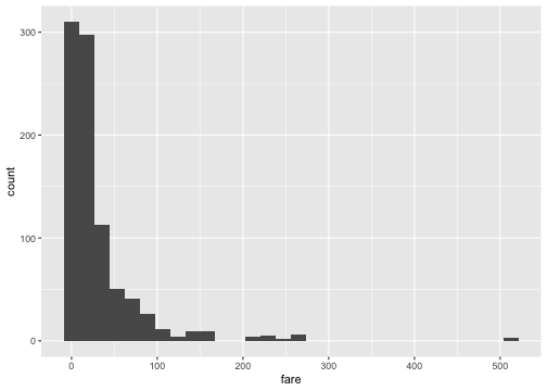<!-- --> ] --- ## What is this warning? ``` ## `stat_bin()` using `bins = 30`. Pick better value with `binwidth`. ``` <img src="01c-visualizing-data_files/figure-html/unnamed-chunk-35-1.png" style="display: block; margin: auto;" /> --- ```r ggplot(data = titanic, aes(x = fare)) + * geom_histogram(binwidth = 15) ``` <img src="01c-visualizing-data_files/figure-html/unnamed-chunk-36-1.png" style="display: block; margin: auto;" /> --- class: middle .panelset[ .panel[.panel-name[binwidth = 15] .left-panel[ ] <img src="01c-visualizing-data_files/figure-html/unnamed-chunk-37-1.png" style="display: block; margin: auto;" /> ] .panel[.panel-name[binwidth = 50] <img src="01c-visualizing-data_files/figure-html/unnamed-chunk-38-1.png" style="display: block; margin: auto;" /> ] .panel[.panel-name[binwidth = 100] <img src="01c-visualizing-data_files/figure-html/unnamed-chunk-39-1.png" style="display: block; margin: auto;" /> ] ] --- class: middle center [There is no "best" number of bins](https://en.wikipedia.org/wiki/Histogram#Number_of_bins_and_width) --- class: middle center .font150[ 🌈 ] Pick your favorite color(s) from the list at: [bit.ly/colors-r](https://bit.ly/colors-r) --- ```r ggplot(data = titanic, aes(x = fare)) + geom_histogram(binwidth = 15, * color = "white") ``` <img src="01c-visualizing-data_files/figure-html/unnamed-chunk-40-1.png" style="display: block; margin: auto;" /> --- ```r ggplot(data = titanic, aes(x = fare)) + geom_histogram(binwidth = 15, * fill = "darkred") ``` <img src="01c-visualizing-data_files/figure-html/unnamed-chunk-41-1.png" style="display: block; margin: auto;" /> --- ```r ggplot(data = titanic, aes(x = fare)) + geom_histogram(binwidth = 15, * color = "white", * fill = "darkred") ``` <img src="01c-visualizing-data_files/figure-html/unnamed-chunk-42-1.png" style="display: block; margin: auto;" /> --- class: inverse middle center .font75[Visualizing Two Categorical Variables] --- ## Stacked Bar-Plot .pull-left[ ```r ggplot(data = titanic, aes(x = pclass, * fill = survived)) + geom_bar() ``` ] .pull-right[ 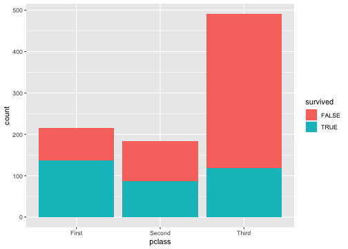<!-- --> ] --- ## Standardized Bar Plot .pull-left[ ```r ggplot(data = titanic, aes(x = pclass, fill = survived)) + * geom_bar(position = "fill") ``` ] .pull-right[ 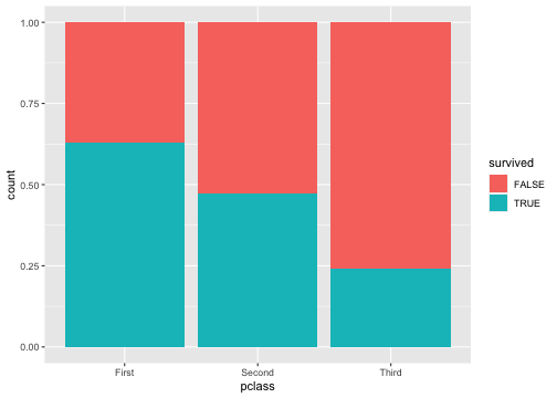<!-- --> ] .footnote[Note that y-axis is no longer count but we will learn how to change that later.] --- ## Dodged Bar Plot .pull-left[ ```r ggplot(data = titanic, aes(x = pclass, fill = survived)) + * geom_bar(position = "dodge") ``` ] .pull-right[ 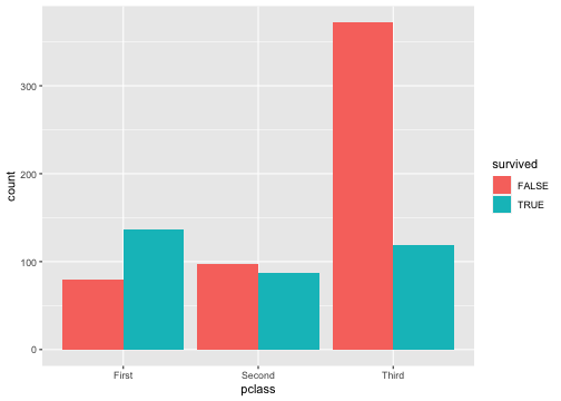<!-- --> ] .footnote[Note that y-axis is no longer count but we will change that later.] --- ## New Data <img src="img/penguins.png" width="667" style="display: block; margin: auto;" /> .footnote[Artwork by [@allison_horst](https://twitter.com/allison_horst) ] --- ## New Data ```r glimpse(penguins) ``` ``` ## Rows: 344 ## Columns: 8 ## $ species <fct> Adelie, Adelie, Adelie, Adelie, Adelie, Adelie, Adel… ## $ island <fct> Torgersen, Torgersen, Torgersen, Torgersen, Torgerse… ## $ bill_length_mm <dbl> 39.1, 39.5, 40.3, NA, 36.7, 39.3, 38.9, 39.2, 34.1, … ## $ bill_depth_mm <dbl> 18.7, 17.4, 18.0, NA, 19.3, 20.6, 17.8, 19.6, 18.1, … ## $ flipper_length_mm <int> 181, 186, 195, NA, 193, 190, 181, 195, 193, 190, 186… ## $ body_mass_g <int> 3750, 3800, 3250, NA, 3450, 3650, 3625, 4675, 3475, … ## $ sex <fct> male, female, female, NA, female, male, female, male… ## $ year <int> 2007, 2007, 2007, 2007, 2007, 2007, 2007, 2007, 2007… ``` --- <img src="img/penguin_bill.png" width="1036" style="display: block; margin: auto;" /> .footnote[Artwork by [@allison_horst](https://twitter.com/allison_horst) ] --- class: middle inverse .font75[Visualizing a single numerical and single categorical variable.] --- class: middle .panelset[ .panel[ .panel-name[Plot] ``` ## Warning: Removed 2 rows containing non-finite values (stat_ydensity). ``` <img src="01c-visualizing-data_files/figure-html/unnamed-chunk-52-1.png" style="display: block; margin: auto;" /> ] .panel[ .panel-name[English] - Create a ggplot using the `penguins` data frame. - Map the `species` to the x-axis and `bill_length_mm` to the y-axis. - Add a layer of a violin plot. ] .panel[ .panel-name[R] ```r ggplot(penguins, aes(x = species, y = bill_length_mm)) + geom_violin() ``` ] ] --- class: middle .panelset[ .panel[ .panel-name[Plot] ``` ## Warning: Removed 2 rows containing non-finite values (stat_ydensity). ``` <img src="01c-visualizing-data_files/figure-html/unnamed-chunk-54-1.png" style="display: block; margin: auto;" /> ] .panel[ .panel-name[English] - Create a ggplot using the `penguins` data frame. - Map the `species` to the x-axis and `bill_length_mm` to the y-axis. - Add a layer of a box plot. ] .panel[ .panel-name[R] ```r ggplot(penguins, aes(x = species, y = bill_length_mm)) + geom_violin() ``` ] ] --- class: middle .pull-left[ <!-- --> ] .pull-right[ <!-- --> ] .footnote[Note: violin plots display densities, not counts!] --- class: middle .pull-left[ <!-- --> ] .pull-right[ <!-- --> ] .footnote[Note: violin plots display densities, not counts!] --- class: inverse middle .font75[Visualizing Two Numerical Variables] --- .left-panel[ ```r ggplot(penguins, aes(x = bill_depth_mm, y = bill_length_mm)) + geom_point() ``` ] .right-panel[ ``` ## Warning: Removed 2 rows containing missing values (geom_point). ``` <!-- --> ] --- class: middle inverse .font75[Considering More Than Two Variables] --- .left-panel[ ```r ggplot(penguins, aes(x = bill_depth_mm, y = bill_length_mm, color = species)) + geom_point() ``` ] .right-panel[ ``` ## Warning: Removed 2 rows containing missing values (geom_point). ``` <!-- --> ] --- .left-panel[ ```r ggplot(penguins, aes(x = bill_depth_mm, y = bill_length_mm, shape = species)) + geom_point() ``` ] .right-panel[ ``` ## Warning: Removed 2 rows containing missing values (geom_point). ``` <!-- --> ] --- .left-panel[ ```r ggplot(penguins, aes(x = bill_depth_mm, y = bill_length_mm, shape = species)) + geom_point() ``` ] .right-panel[ ``` ## Warning: Removed 2 rows containing missing values (geom_point). ``` <!-- --> ] --- .left-panel[ ```r ggplot(penguins, aes(x = bill_depth_mm, y = bill_length_mm, shape = species, color = species)) + geom_point() ``` ] .right-panel[ ``` ## Warning: Removed 2 rows containing missing values (geom_point). ``` <!-- --> ] --- .left-panel[ ```r ggplot(penguins, aes(x = bill_depth_mm, y = bill_length_mm, shape = species, color = species, size = body_mass_g)) + geom_point() ``` ] .right-panel[ ``` ## Warning: Removed 2 rows containing missing values (geom_point). ``` <!-- --> ] --- <img src="img/ggplot-summary.jpeg" width="95%" /> --- class: middle .panelset[ .panel[ .panel-name[Plot] <img src="01c-visualizing-data_files/figure-html/unnamed-chunk-73-1.png" style="display: block; margin: auto;" /> ] .panel[ .panel-name[English] - Using the `penguins` data, - Map `bill depth` to x-axis, `bill length` to y-axis, `species` to shape and color. - Add a layer of points and set the size of the points to 4. ] .panel[ .panel-name[R] ```r ggplot(penguins, aes(x = bill_depth_mm, y = bill_length_mm, shape = species, color = species)) + geom_point(size = 4) ``` ] ] --- class: middle ## Labs .panelset[ .panel[ .panel-name[Plot] <img src="01c-visualizing-data_files/figure-html/unnamed-chunk-75-1.png" style="display: block; margin: auto;" /> ] .panel[ .panel-name[English] - Using the `penguins` data, - Map `bill depth` to x-axis, `bill length` to y-axis, `species` to shape. - Add a layer of points and set the size of the points to 4. - .highlight-text[Add labels to x-axis (Bill Depth(mm)), y-axis (Bill Length(mm)), and the title of the plot (Palmer Penguins).] .panel[ .panel-name[R] ```r ggplot(penguins, aes(x = bill_depth_mm, y = bill_length_mm, shape = species, color = species)) + geom_point(size = 4) + * labs(x = "Bill Depth (mm)", * y = "Bill Length (mm)", * title = "Palmer Penguins") ``` ] ] ] --- class: middle .left-panel[ ```r ggplot(penguins, aes(x = bill_depth_mm, y = bill_length_mm, shape = species, color = species)) + geom_point() + labs(x = "Bill Depth (mm)", y = "Bill Length (mm)", title = "Palmer Penguins") + * theme_bw() ``` ] .right-panel[ 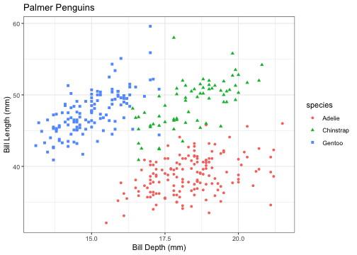<!-- --> ] --- class: middle ## Themes .panelset[ .panel[ .panel-name[`theme_gray()`] <img src="01c-visualizing-data_files/figure-html/unnamed-chunk-79-1.png" style="display: block; margin: auto;" /> ] .panel[ .panel-name[`theme_bw()`] <img src="01c-visualizing-data_files/figure-html/unnamed-chunk-80-1.png" style="display: block; margin: auto;" /> ] .panel[ .panel-name[`theme_classic()`] <img src="01c-visualizing-data_files/figure-html/unnamed-chunk-81-1.png" style="display: block; margin: auto;" /> ] .panel[ .panel-name[`theme_dark()`] <img src="01c-visualizing-data_files/figure-html/unnamed-chunk-82-1.png" style="display: block; margin: auto;" /> ] .panel[ .panel-name[`theme_minimal()`] <img src="01c-visualizing-data_files/figure-html/unnamed-chunk-83-1.png" style="display: block; margin: auto;" /> ] .panel[ .panel-name[`theme_void()`] <img src="01c-visualizing-data_files/figure-html/unnamed-chunk-84-1.png" style="display: block; margin: auto;" /> ] ] --- class: middle .left-panel[ ```r ggplot(penguins, aes(x = bill_depth_mm, y = bill_length_mm, shape = species, color = species)) + geom_point() + labs(x = "Bill Depth (mm)", y = "Bill Length (mm)", title = "Palmer Penguins") + theme_bw() + * theme(text = element_text(size=20)) ``` ] .right-panel[ <!-- --> ] --- class: middle ```r ?theme ``` --- class: middle .left-panel[ ```r ggplot(penguins, aes(x = bill_depth_mm, y = bill_length_mm, shape = species, color = species)) + geom_point(size = 4) + * facet_grid(.~species) ``` ] .right-panel[ <img src="01c-visualizing-data_files/figure-html/unnamed-chunk-89-1.png" style="display: block; margin: auto;" /> ] --- class: middle .left-panel[ ```r ggplot(penguins, aes(x = bill_depth_mm, y = bill_length_mm, shape = species, color = species)) + geom_point(size = 4) + * facet_grid(species~.) ``` ] .right-panel[ <img src="01c-visualizing-data_files/figure-html/unnamed-chunk-91-1.png" style="display: block; margin: auto;" /> ] --- class: middle .left-panel[ ```r ggplot(penguins, aes(x = bill_depth_mm, y = bill_length_mm)) + geom_point() + * xlim(0, 30) + * ylim(0,70) ``` ] .right-panel[ <!-- --> ] --- class: middle ## code style [The tidyverse style guide](https://style.tidyverse.org/ggplot2.html) has the following convention for writing ggplot2 code. Similar to the piper operator`%>%`, the plus sign for adding layers `+` always has a space before it and is followed by a new line. The new line is indented by two spaces. RStudio does this automatically for you. --- class: middle [Top Ten Dos and Don't for Charts and Graphs](https://guides.lib.uci.edu/datavis/do) --- class: middle Check out [the ggplot flipbook](https://evamaerey.github.io/ggplot_flipbook/ggplot_flipbook_xaringan.html#1) for some inspiration. Find your favorite new function/feature. Share it with your neighbor. --- class: middle ## ggplot extensions - [`patchwork`](https://patchwork.data-imaginist.com/) combining plots into a single plot - [`gganimate`](https://gganimate.com/) animated graphics - [`ggthemes`](https://rafalab.github.io/dsbook/ggplot2.html#add-on-packages) additional set of themes - [`ggtext`](https://wilkelab.org/ggtext/) improved text rendering support for ggplot2 There are [more extensions](https://exts.ggplot2.tidyverse.org/gallery/) --- class: middle center inverse .font75[Making Accessible Visualizations] --- class: middle [Color blindness simulation](https://www.color-blindness.com/coblis-color-blindness-simulator/): red-blind/protanopia <img src="img/red-blind.png" width="60%" style="display: block; margin: auto;" /> --- class: middle [Color blindness simulation](https://www.color-blindness.com/coblis-color-blindness-simulator/): green-blind/deuteranopia <img src="img/green-blind.png" width="60%" style="display: block; margin: auto;" /> --- class: middle [Color blindness simulation](https://www.color-blindness.com/coblis-color-blindness-simulator/): blue-blind/tritanopia <img src="img/blue-blind.png" width="60%" style="display: block; margin: auto;" /> --- class: middle ```r palette.colors(palette = "Okabe-Ito") ``` ``` ## black orange skyblue bluishgreen yellow ## "#000000" "#E69F00" "#56B4E9" "#009E73" "#F0E442" ## blue vermillion reddishpurple gray ## "#0072B2" "#D55E00" "#CC79A7" "#999999" ``` [Okabe-Ito color palette](https://jfly.uni-koeln.de/color/) allows us to make figures that are colorblind friendly. You can use the HEX code printed for selecting colors. --- class: middle .left-panel[ ```r ggplot(penguins, aes(x = bill_depth_mm, y = bill_length_mm, shape = species, color = species)) + geom_point(size = 4) + facet_grid(species~.) + * scale_color_manual(values = * c("#E69F00", * "#009E73", * "#56B4E9")) ``` ] .right-panel[ <!-- --> ]