Categorical Data Analysis

Author: Jose Toledo Luna

Co-author: Jessica Jaynes

Overview

Part 1: Basic Probability Review and Common Discrete Distributions

Part 2: Chi-square test of independence

Part 3: Chi-square goodness of fit test

Part 1: Basic Probability Review

Definitions

The sample space is the set of all the possible outcomes of an experiment. A sample space will be denoted by \(S\).

Any subset of of a sample space is called an event.

Example

Flip a coin three times. The sample space is then \[ S = \{HHH, HHT, HTH, THH, HTT, THT, TTH, TTT \} \] There are eight possible outcomes in this experiment

Example

Define the event \(\,A=\) observing two heads in three coin tosses.

Recall, the sample space is \[ S = \{HHH, HHT, HTH, THH, HTT, THT, TTH, TTT \} \]

Then the probability of observing this event is \[ P(A) = \frac{|A|}{|S|} = \frac{3}{8} \] where \(|\cdot|\) denotes the cardinality of a set

Random Variables

A random variable, usually denoted by an upper case \(X\), is a variable whose possible values are numerical outcomes of a random phenomenon (Experiment)

There are two types of random variables, discrete and continuous.

For today’s discussion we will only focus on discrete random variables

A random variable \(X\) is said to be discrete if it can assume only a finite or countably infinite number of distinct values

Bernoulli Distribution

The Bernoulli distribution is a discrete probability distribution that models a single binary outcome, often denoted as “success” or “failure”.

In order to model an experiment through a Bernoulli distribution, all of the following conditions must hold

• There are only two possible outcomes for an experiment or trial: a success and the other as a failure.
• The probability of success, denoted as \(p\), represents the likelihood of the desired outcome occurring. The probability of failure is calculated as \(1 - p\).
• Each trial is assumed to be independent, meaning that the outcome of one trial does not affect the outcome of any other trial.
• The probability of success remains constant across all trials.

Bernoulli Probability Mass Function

Given a random variable \(X\) follows a Bernoulli distribution, \(X \sim Ber(p)\), then the probability mass function is given by \[ P(X = k) = p^k\, (1-p)^{1-k} \] for \(k \in \{0,1\}\) and \(p \in [0,1]\)

• \(\mathbb{E}(X) = p\)
• \(Var(X) = p(1-p)\)

Binomial Distribution

The binomial distribution is a probability distribution that models the number of successes in a fixed number of independent Bernoulli trials.

Binomial Coefficient

The number of of combinations of \(n\) objects taken \(k\) at a time is the number of subsets, each of size \(k,\) that can be formed from the \(n\) objects is denoted by \[ \binom{n}{k} = \frac{n !}{k! (n-k)!} \] for a pair of integers \(n \geq k \geq 0\). This is known as the binomial coefficient

Example: Choosing 3 desserts from a menu of 10 items \(\binom{10}{3} = \frac{10!}{3! (10-3)!} = 120\)

Binomial Probability Mass Function

Given a random variable \(X\) following a binomial distribution, \(X \sim B(n,p)\). The probability of obtaining exactly \(k\) successes in \(n\) independent Bernoulli trials is given by the following probability mass function \[ P(X = k) = \binom{n}{k} \, p^k\, (1-p)^{n-k} \] for a pair of integers \(n \geq k \geq 0\) and \(p \in [0,1]\)

Interpretation: The probability of having \(k\) successes is \(p^k\) and the probability of having \((n-k)\) failures is \((1-p)^{n-k}\).

The \(k\) successes can occur at any position among the \(n\) trials, and there are \(\binom{n}{k}\) ways to distribute the successes in the sequence of trials.

Binomial Distribution

In order to model an experiment through a binomial distribution, all of the following conditions must be satisfied

• There are a fixed number of \(n\) trials
• The trials are independent of one another
• For each trial, the event of interest represents one of two outcomes (success or failure)
• The probability of “success” \(p\) is the same on each trial

The Bernoulli distribution is a special case of the binomial distribution with \(n=1\):

• \(\mathbb{E}(X) = np\)
• \(Var(X) = np(1-p)\)

Binomial Distribution: Example

Consider (again) the scenario of flipping a fair coin three times.

\[ S = \{HHH, HHT, HTH, THH, HTT, THT, TTH, TTT \} \] The event \(\,A\) = observing two heads in three coin tosses, then \(P(A) = \frac{|A|}{|S|} = \frac{3}{8}\)

Given the following conditions,

• We have a fixed number of trials, which is three coin flips
• Each coin flip is assumed to be independent of the others. The outcome of one flip does not affect the outcome of the other flips.
• In this case, the two possible outcomes are heads (H) and tails (T).
• Assuming a fair coin, the probability of getting heads (success) on any single flip is 0.5, and the probability of getting tails (failure) is also 0.5

we can model the number of heads obtained in three coin flips using a binomial distribution

Let \(\, X=\) number of heads in three fair coin tosses. Since the coin is fair, the probability of obtaining heads (success) is \(p = \frac{1}{2}\). Therefore, \(\,X\sim B\left(n=3,p=\frac{1}{2}\right)\) and we are interested in observing two heads

\[ \begin{align*} P(X = k) &= \binom{n}{k} \, p^k\, (1-p)^{n-k} \\[2pt] P(X=2) &= \binom{3}{2} \left(\frac{1}{2} \right)^2 \left(\frac{1}{2} \right)^{3-2} \\[2pt] &= \frac{3!}{2! \,1!} \left(\frac{1}{2} \right)^3 \\[2pt] &= \frac{3}{8} \end{align*} \]

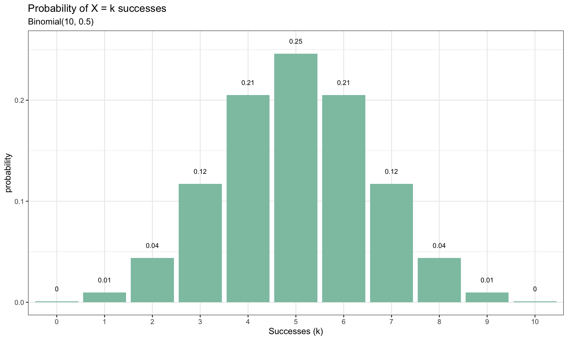
While the previous example was simple, consider a scenario where you are flipping a coin ten times. In such cases, it becomes impractical and time-consuming to manually list out all the possible combinations of coin tosses \((|S| = 1024)\)

\(X \sim B(n=10,p=\frac{1}{2})\), and we are interested in calculating the probability of observing four heads. This can easily be done

\[ \begin{align*} P(X = 4) &= \binom{10}{4} \left(\frac{1}{2}\right)^{4} \left( \frac{1}{2} \right)^{10-4} \\[5pt] &= \frac{10!}{4!(10-6)!} \left( \frac{1}{2} \right)^{10} \\[5pt] &= \frac{210}{1024} \end{align*} \]

We can calculate the remaining probabilities of obtaining \(k\) heads

Show code

dat <- tibble(heads = 0:10, prob = dbinom(x = 0:10, size = 10, prob = 0.5))

ggplot(dat,aes(x = factor(heads), y = prob)) +
  geom_col(fill = '#8dc4b0') +
  geom_text(aes(label = round(prob,2), y = prob + 0.01),
    position = position_dodge(0.9),
    size = 3,vjust = 0) +
  labs(title = "Probability of X = k successes",
       subtitle = "Binomial(10, 0.5)",
       x = "Successes (k)",y = "probability")

Distributions in R

Each probability distribution in R is associated with four functions which follow a naming convention

• the probability density/mass function always begins with ‘d’,
• the cumulative distribution function always begins with ‘p’,
• the inverse cumulative distribution (or quantile function) always beings with ‘q’,
• function that produces random variables always begins with ‘r’.

Below is an example using the Binomial distribution

Function	Description	Usage
dbinom	Binomial density (Probability Mass Function)	dbinom(x=1,size=10,prob=0.5)
pbinom	Binomial distribution (Cumulative Distribution Function)	pbinom(q=4,size=10,prob=0.5)
qbinom	Quantile function of the Binomial distribution	qbinom(p=0.5,size=10,prob=0.5)
rbinom	Binomial random number generation	rbinom(n=10,size=10,prob=0.5)

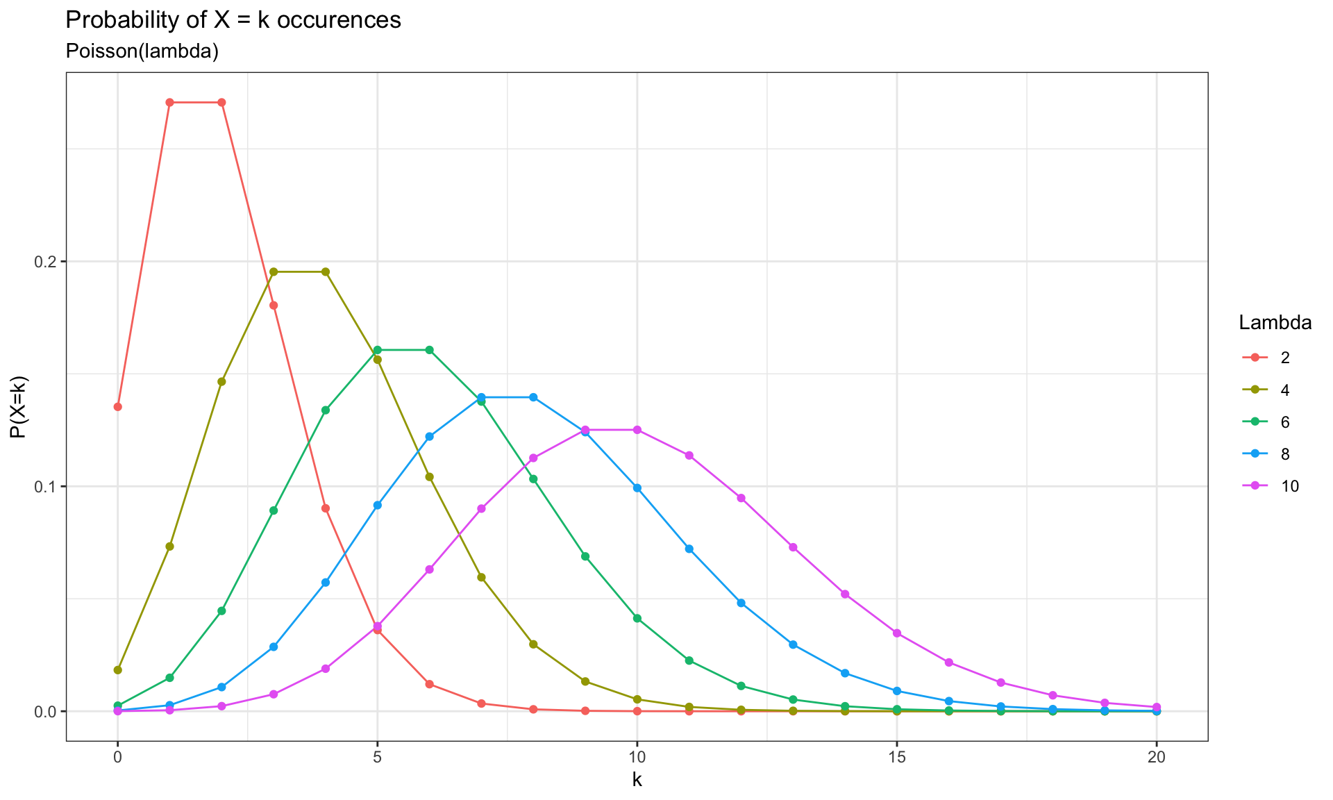
Poisson Distribution

The Poisson distribution helps us understand the frequency of events occurring within a specific time or space interval. It provides the probability of observing a certain number of events when the average rate of occurrence is known.

Poisson Probability Mass Function

Given a random variable \(X\) following a Poisson distribution, \(\,X \sim Pois(\lambda)\), with parameter \(\lambda >0\). The probability of observing \(k\) occurrences is given by the following probability mass function \[ P(X = k) = \frac{\lambda^k e^{-\lambda}}{k!} \] for \(k = (0,1,2,\dots)\)

If \(\,X \sim Pois(\lambda)\), then both expectation \(\mathbb{E}(X)\) and \(Var(X)\) are equal to \(\lambda\), i.e., the spread or variability of the Poisson distribution is directly determined by the average rate \((\lambda)\) of an event occurrence.

Show code

x_vals <- 0:20
lambda_vals <- seq(2,10,2)

p_dat <- map_df(lambda_vals, ~ tibble(
  l = paste(.),
  x = x_vals,
  y = dpois(x_vals, .)
))

ggplot(p_dat, aes(x, y, color = factor(l, levels = lambda_vals))) +
  geom_line() +
  geom_point(data = p_dat, 
             aes(x, y, color = factor(l, levels = lambda_vals))) +
  labs(title = "Probability of X = k occurences",
       subtitle = "Poisson(lambda)",
       x = "k",y = 'P(X=k)',color = "Lambda")

For Poisson distribution the following conditions must be considered:

• The events of occurrences must be independent of each other
• The events must occur at a constant average rate throughout the specified interval
• It is important to ensure that the average rate of occurrence is relatively low, so that multiple events happening simultaneously or in quick succession is unlikely

Poisson Distribution: Example

Consider a scenario where you have a service facility, such as a call center, or helpdesk, and you want to model the number of customers arriving at the facility during a specific time period

Let’s say from previous data on customer arrivals you find that, on average, you receive 10 customer arrivals per hour

1. What is \(\,\lambda\) ?
2. What is the probability of having exactly 8 customers arrive during the next hour ?

Part 2: \(\chi^2\) Test of Independence

The \(\chi^2\) test of independence is a statistical test used to determine whether there is a significant association between two categorical variables.

It helps to assess whether the occurrence of one categorical variable is related to the occurrence of another categorical variable

Example: How important is it to ask pointed questions?

The following is example is taken from Chapter 18 of Introduction to Modern Statistics.

“We all buy used products – cars, computers, textbooks, and so on – and we sometimes assume the sellers of those products will be forthright about any underlying problems with what they’re selling. This is not something we should take for granted. Researchers recruited 219 participants in a study where they would sell a used iPod176 that was known to have frozen twice in the past. The participants were incentivized to get as much money as they could for the iPod since they would receive a 5% cut of the sale on top of $10 for participating. The researchers wanted to understand what types of questions would elicit the seller to disclose the freezing issue.”

Example: How important is it to ask pointed questions?

“Unbeknownst to the participants who were the sellers in the study, the buyers were collaborating with the researchers to evaluate the influence of different questions on the likelihood of getting the sellers to disclose the past issues with the iPod. The scripted buyers started with “Okay, I guess I’m supposed to go first. So you’ve had the iPod for 2 years …” and ended with one of three questions:”

• General: What can you tell me about it ?
• Positive Assumption: It doesn’t have any problems, does it ?
• Negative Assumption: What problem does it have ?

“The question is the treatment given to the sellers, and the response is whether the question prompted them to disclose the freezing issue with the iPod.”

Example: How important is it to ask pointed questions?

The ask dataset for this experiment can be found in the openintro R package.

glimpse(ask)

Rows: 219
Columns: 3
$ question_class <chr> "general", "pos_assumption", "pos_assumption", "neg_ass…
$ question       <chr> "What can you tell me about it?", "It doesn't have any …
$ response       <chr> "hide", "hide", "disclose", "disclose", "hide", "disclo…

count(ask, question_class)

# A tibble: 3 × 2
  question_class     n
  <chr>          <int>
1 general           73
2 neg_assumption    73
3 pos_assumption    73

count(ask, response)

# A tibble: 2 × 2
  response     n
  <chr>    <int>
1 disclose    61
2 hide       158

Two-way Contingency Table

ask_two_way <- openintro::ask |> 
  select(question_class, response) |> 
  table() |> 
  addmargins()

	Disclose	Hide	Total
General	2	71	73
Negative_assumption	36	37	73
Positive_assumption	23	50	73
Total	61	158	219

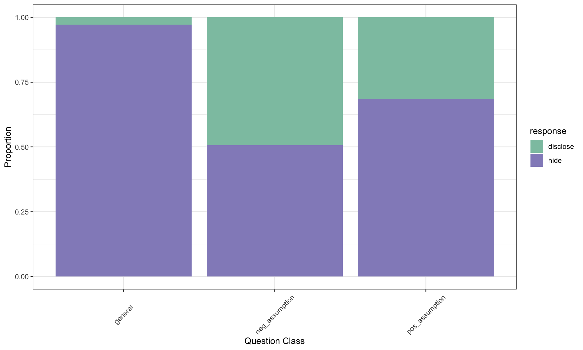
To perform the \(\chi^2\) test of independence, the data is organized in a contingency table (shown above). This table displays the frequencies of the different combinations of categories for the two variables

Show code

openintro::ask |> 
  ggplot() +
  aes(x = question_class, fill = response) +
  geom_bar(position = "fill") +
  scale_fill_manual(values=c('#8dc4b0','#948DC4')) +
  theme(axis.text.x = element_text(angle = 45,vjust = .5)) +
  labs(x = "Question Class",
       y = "Proportion")

If there were no relationship, we would expect to see the purple bars reaching to the same height, regardless of the question class

Expected Counts

To calculate the expected count for the \(i^{th}\) row and \(j^{th}\) column, compute \[ \text{Expected Count}_{\,row \, i,\, \;col \, j } = \frac{ (\text{row}\,\; i \; \text{total}) \times (\text{column}\,\; j \; \text{total}) }{ \text{table total} } \]

	Disclose	Hide	Total
General	2	71	73
Negative_assumption	36	37	73
Positive_assumption	23	50	73
Total	61	158	219

\(\text{Expected Count}_{\,row \, 1,\, \;col \, 1 } =\)

\[ \frac{(\text{row 1 total}) \times (\text{column 1 total}) }{ (\text{table total}) } = \]

\[ \frac{73 \times 61}{219} = 20.33 \]

\(\text{Expected Count}_{\,row \, 1,\, \;col \, 2 } =\)

\[ \frac{(\text{row 1 total}) \times (\text{column 2 total}) }{ (\text{table total}) } = \]

\[ \frac{73 \times 158}{219} = 52.67 \]

Similarly, compute the expected counts for the remaining cells.

Two-way Contingency Table: Observed and Expected Counts

Question Type	Disclose (Expected)	Hide (Expected)	Total
General	2 (20.33)	71 (52.67)	73
Positive assumption	23 (20.33)	50 (52.67)	73
Negative assumption	36 (20.33)	37 (52.67)	73
Total	61	158	219

The \(\chi^2\) test statistic for a two-way table is found by finding the ratio of how far the observed counts are from the expected counts

\(\chi^2\) test-statistic

The test statistic for assessing the independence between two categorical variables

\[ \chi^2 = \sum_{ij} \frac{ (\text{observed count - expected count})^2 }{ \text{expected count} } \] When the null hypothesis is true and the conditions are met, \(\, \chi^2\) has a Chi-squared distribution with \(\, df = (r-1) \times (c-1)\), where \(r=\) number of rows, and \(c=\) number of columns

Conditions:

• Independent observations
• Large samples: At least 5 expected counts in each cell

Question Type	Disclose (Expected)	Hide (Expected)	Total
General	2 (20.33)	71 (52.67)	73
Positive assumption	23 (20.33)	50 (52.67)	73
Negative assumption	36 (20.33)	37 (52.67)	73
Total	61	158	219

row 1, column 1 \[ \frac{(2-20.33)^2}{20.33} = 16.53 \] row 2, column 1 \[ \begin{align*} \frac{(23-20.33)^2}{20.33} &= 0.35 \\ &\vdots \end{align*} \] row 3, column 2 \[ \frac{(37-52.67)^2}{52.67} = 4.66 \]

For each cell use the general formula: \[ \frac{(\text{observed - expected})^2}{\text{expected}} \]

Calculating the \(\chi^2\) Test Statistic

Question Type	Disclose	Hide
General	16.53	6.38
Positive assumption	0.35	0.14
Negative assumption	12.07	4.66

Adding the computed value for each cell gives the \(\chi^2\) test statistic: \[ \chi^2 = 16.53 + 0.53 + \cdots + 4.66 = 40.13 \]

Does the value of the \(\chi^2=40.13\) test statistic indicate that the observed and expected values are really different ?

Or is \(\chi^2 = 40.13\) a value we’d expect to see just due to natural variability.

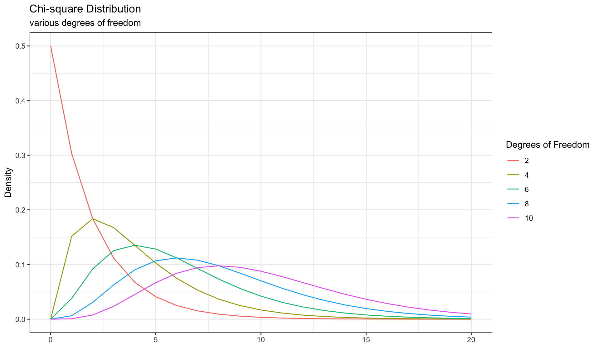
\(\chi^2\) Distribution for Differing Degrees of Freedom

Show code

x_vals <- 0:20
df_vals <- seq(2,10,2)

df_dat <- map_df(df_vals, ~ tibble(
  l = paste(.),
  x = x_vals,
  y = dchisq(x_vals, .)
))

ggplot(df_dat, aes(x, y, color = factor(l, levels = df_vals))) +
  geom_line(data = df_dat, 
             aes(x, y, color = factor(l, levels = df_vals))) +
  labs(title = "Chi-square Distribution",
       subtitle = "various degrees of freedom",
       x = "",y = 'Density',color = "Degrees of Freedom")

The larger the degrees of freedom, the long the right tail extends. The smaller the degrees of freedom, the more peaked the mode on the left becomes

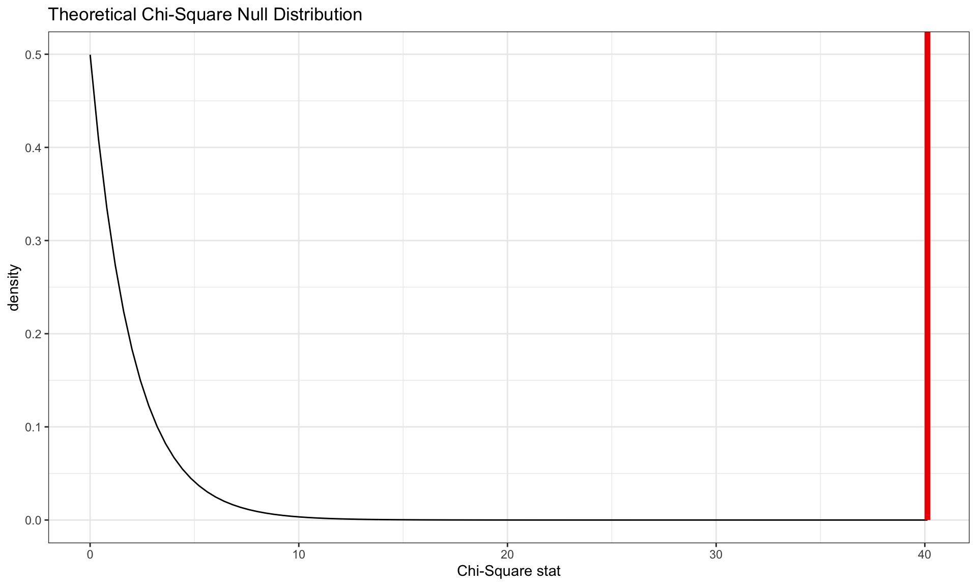
We need to understand the variability in the values of the \(\chi^2\) statistic we would expect to see if the null hypothesis was true (i.e, \(\chi^2\) distribution with \(df = (3-2) \times (2-1) = 2\)).

The red vertical line is our observed \(\chi^2=40.13\) test statistic.

We can now compute the \(\,p\)-value and draw a conclusion about whether the question affects the sellers likelihood of reporting the iPod problems:

1 - pchisq(40.13, df = 2)

[1] 1.93144e-09

Using a significance level of \(\, \alpha = 0.05,\) the null hypothesis is rejected since the \(\,p\)-value is smaller.

That is the data provide convincing evidence that the question asked did affect a seller’s likelihood to tell the truth about problems with the iPod.

Test of Independence: Using Infer

The following implementation considers the use of the package infer, which is part of the tidymodels ecosystem.

We will conduct a \(\chi^2\) test of independence to determine whether there is a relationship between the question class and the disclosure/hiding of the problem with the iPod by the participants.

library(infer)
observed_indep_statistic <- openintro::ask |> 
  specify(response ~ question_class) |> 
  hypothesize(null = "independence") |> 
  calculate(stat = "Chisq")

Response: response (factor)
Explanatory: question_class (factor)
Null Hypothesis: independence
# A tibble: 1 × 1
   stat
  <dbl>
1  40.1

The observed \(\chi^2\) statistic is 40.1.

Now we want to compare the observed \(\chi^2 = 40.1\) statistic to a null distribution, generated under the assumption that the question class and the disclosure/hiding of the problem with the iPod are not actually related.

We generate the null distribution using a randomization approach

The randomization approach approximates the null distribution by randomly shuffling the response and explanatory variables. This process ensures that each participant’s question class is paired with a randomly chosen disclosure or hiding of the problem with the iPod from the sample. The purpose is to disrupt any existing association between the two variables

• Code
• Output

First, generate the null distribution using randomization

null_dist_sim <- openintro::ask |> 
  specify(response ~ question_class) |> 
  hypothesize(null = "independence") |> 
  generate(reps = 1000, type = "permute") |> 
  calculate(stat = "Chisq")

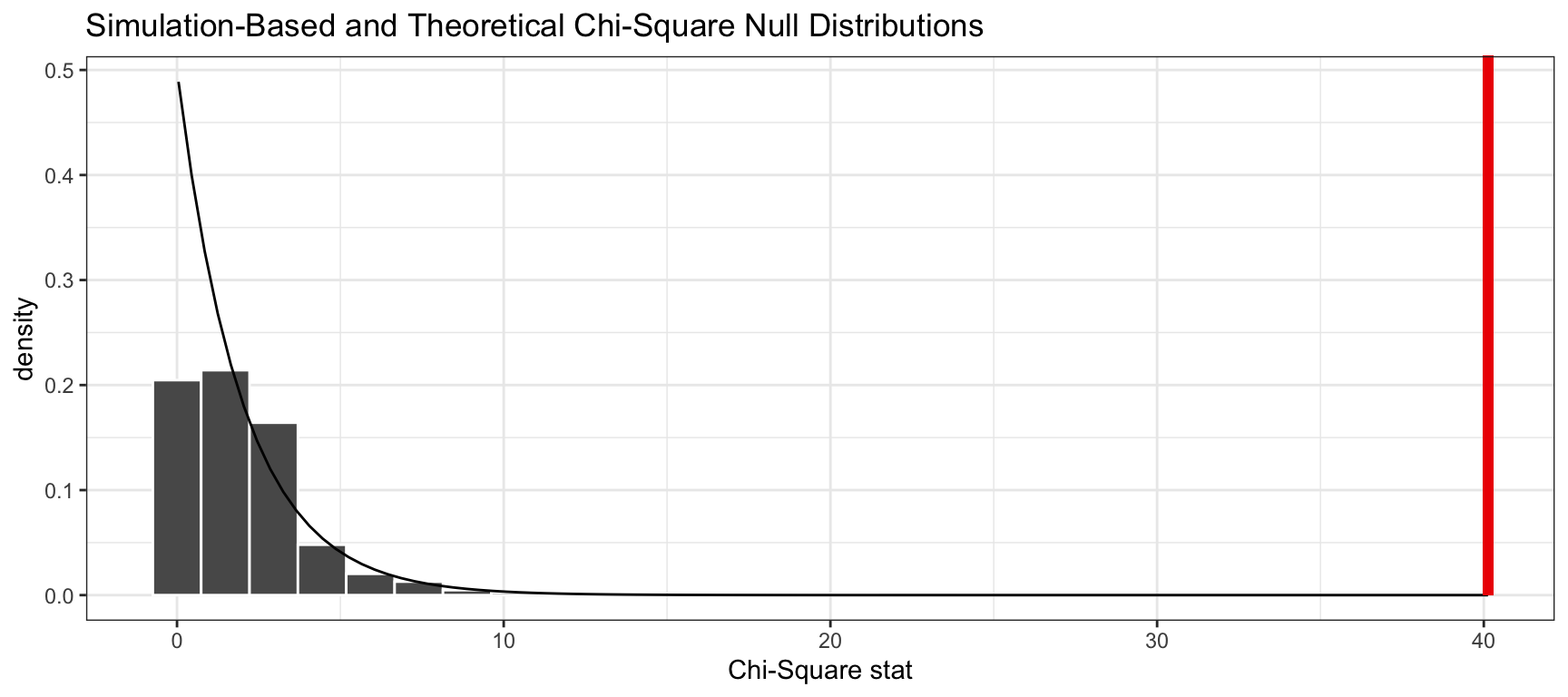
To visualize both the randomization-based and theoretical null distribution, we can pipe the randomization-based null distribution into visualize(), and provide method = "both"

null_dist_sim |> 
  visualize(method = "both") + 
  shade_p_value(observed_indep_statistic,
                direction = "greater")

None of the 1,000 simulations had a \(\chi^2\) value of at least 40.13. In fact, none of the simulated \(\chi^2\) statistics came anywhere close to the observed statistic

Using the simulated null distribution, we can approximate the \(\,p\,\)-value with get_p_value

null_dist_sim |> 
  get_p_value(obs_stat = observed_indep_statistic, direction = "greater")

# A tibble: 1 × 1
  p_value
    <dbl>
1       0

Therefore, if there were really no relationship between the question class and the disclosure/hiding of the problem with the iPod, our approximation of the probability that we would see a statistic as or more extreme than 40.1 is approximately 0.

Equivalently, the theory-based approach to calculate the \(\,p\,\)-value using the true \(\chi^2\) distribution can be obtained using the base R function pchisq.

pchisq(observed_indep_statistic$stat, 
       df = 2, lower.tail = FALSE)

   X-squared 
1.933339e-09 

The infer package provides a wrapper function chisq_test, to carry out \(\chi^2\) test of independence on tidy data.

chisq_test(openintro::ask, response ~ question_class)

# A tibble: 1 × 3
  statistic chisq_df       p_value
      <dbl>    <int>         <dbl>
1      40.1        2 0.00000000193

Part 3: \(\chi^2\) Goodness of Fit

The \(\chi^2\) goodness of fit test is a statistical test used to determine whether observed categorical data follows an expected distribution or conforms to a specified theoretical distribution.

It assesses whether there is a significant difference between the observed frequencies and the expected frequencies for different categories or group

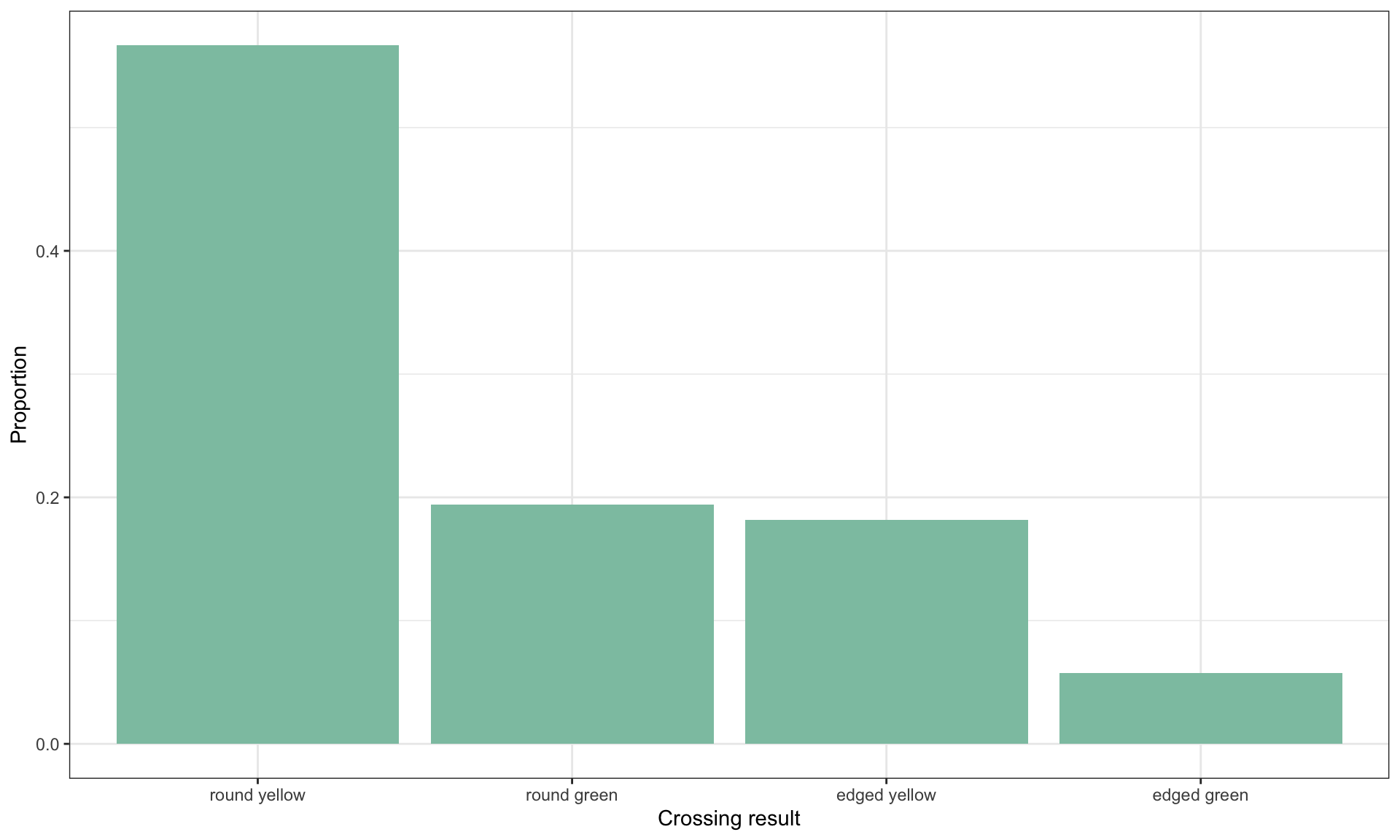
Gregor Mendel’s Experiments

From (1822-1884) Gregor Mendel conducted crossing experiments with pea plants of different shapes and color. Let us look at the outcome of a pea crossing experiment with the following results:

Show code

crossing_peas <- tibble::tibble(cross_result = 
                                  rep(c('round yellow', 'round green',
                                        'edged yellow','edged green'),
                                      c(315,108,101,32) )) |> 
  mutate(cross_result = as.factor(cross_result))

cross_result	Freq
edged green	32
edged yellow	101
round green	108
round yellow	315

Show code

positions <- c('round yellow', 'round green','edged yellow','edged green')

crossing_peas |>
  count(cross_result) |> 
  mutate(proportion = n/sum(n)) |> 
  ggplot() +
  aes(x = cross_result, y= proportion) +
  geom_bar(stat='identity',fill = '#8dc4b0') +
  scale_x_discrete(limits = positions)+
  labs(x = "Crossing result",
       y = "Proportion")

Mendel had the hypothesis that the four different types occur in proportions of 9:3:3:1, that is \[ p_{\text{round-yellow}} = \frac{9}{16}, \, p_{\text{round-green}} = \frac{3}{16}, \, p_{\text{edged-yellow}} = \frac{3}{16}, \, p_{\text{edged-green}} = \frac{1}{16}, \]

Mendel’s hypothesis is then

\[ H_0: \, p_{\text{round-yellow}} = \frac{9}{16}, \, p_{\text{round-green}} = \frac{3}{16}, \, p_{\text{edged-yellow}} = \frac{3}{16}, \, p_{\text{edged-green}} = \frac{1}{16}, \]

\[ H_a: \ p_{\text{round-yellow}} \neq \frac{9}{16}, \, p_{\text{round-green}} \neq \frac{3}{16}, \, p_{\text{edged-yellow}} \neq \frac{3}{16}, \, p_{\text{edged-green}} \neq \frac{1}{16}, \]

The alternative simply states the proportions of the four different outcomes of a pea crossing experiment is not 9:3:3:1

Goodness of Fit: Using Infer

First, to carry out this hypothesis test, we need to calculate out observed statistic

observed_gof_statistic <- crossing_peas |> 
  specify(response = cross_result) |> 
  hypothesize(null = "point",
              p = c("round yellow" = 9/16,
                    "round green" = 3/16,
                    "edged yellow" = 3/16,
                    "edged green" = 1/16)) |> 
  calculate(stat = "Chisq")

Response: cross_result (factor)
Null Hypothesis: point
# A tibble: 1 × 1
   stat
  <dbl>
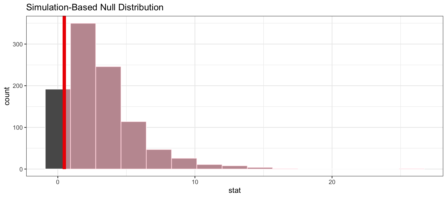
1 0.470

Now we want to compare the observed \(\chi^2 =0.47\) statistic to a null distribution, generated under the assumption that the proportions of the four different outcomes of a pea crossing experiment is 9:3:3:1

• Code
• Output

First, generate the null distribution using simulation

null_dist_gof <- crossing_peas |> 
  specify(response = cross_result) |> 
  hypothesize(null = "point",
              p = c("round yellow" = 9/16,
                    "round green" = 3/16,
                    "edged yellow" = 3/16,
                    "edged green" = 1/16)) |> 
  generate(reps = 1000, type = "draw") |> 
  calculate(stat = "Chisq")

To get a sense for what these distributions look like, and where our observed statistic falls, we can use visualize()

null_dist_gof |> 
  visualize() + 
  shade_p_value(observed_gof_statistic,
                direction = "greater")

The statistic seems like it would be quite likely if the proportions of the four different outcomes of a pea crossing experiment is 9:3:3:1.

Using the simulated null distribution, we can approximate the \(\,p\,\)-value with get_p_value

# A tibble: 1 × 1
  p_value
    <dbl>
1   0.908

Thus, if the proportions of the four different outcomes of a pea crossing experiment is 9:3:3:1, our approximation of the probability that we would see a distribution like the one we did is approximately 0.908

To calculate the \(p\)-value using the true \(\chi^2\) distribution, we can use the pchisq function from base R

pchisq(observed_gof_statistic$stat, df = 3, lower.tail = FALSE)

[1] 0.9254259

The infer package provides a wrapper function chisq_test, to carry out \(\chi^2\) goodness of fit tests on tidy data

chisq_test(crossing_peas, 
           response = cross_result, 
1           p = c("edged green" = 1/16,
                 "edged yellow" = 3/16,
                 "round green" = 3/16,
                 "round yellow" = 9/16))

1

If response is a factor, then list the proportions of the levels in the order of levels(response)

# A tibble: 1 × 3
  statistic chisq_df p_value
      <dbl>    <dbl>   <dbl>
1     0.470        3   0.925

Thus, we do not have sufficient evidence to suggest Mendel’s hypothesis that the four different types occur in proportions of 9:3:3:1 is not wrong. That is we fail to reject the null hypothesis.

(This does not mean we accept Mendel’s hypothesis)