Logistic Regression
Note that examples in this lecture a modified version of Chapter 13 of Bayes Rules! book.
\[Y = \begin{cases} \text{ Yes rain} & \\ \text{ No rain} & \\ \end{cases} \;\]
\[\begin{split} X_1 & = \text{ today's humidity at 9am (percent)} \\ \end{split}\]
Packages
Data
data(weather_perth)
weather <- weather_perth %>%
  select(day_of_year, raintomorrow, humidity9am,
         humidity3pm, raintoday)
glimpse(weather)
Rows: 1,000
Columns: 5
$ day_of_year <dbl> 45, 11, 261, 347, 357, 254, 364, 293, 304, 231, 313, 208,…
$ raintomorrow <fct> No, No, Yes, No, No, No, No, No, Yes, Yes, No, No, No, No…
$ humidity9am <int> 55, 43, 62, 53, 65, 84, 48, 51, 47, 90, 53, 87, 83, 96, 8…
$ humidity3pm <int> 44, 16, 85, 46, 51, 59, 43, 34, 47, 57, 42, 46, 55, 56, 5…
$ raintoday <fct> No, No, No, No, No, Yes, No, No, Yes, Yes, No, No, Yes, Y…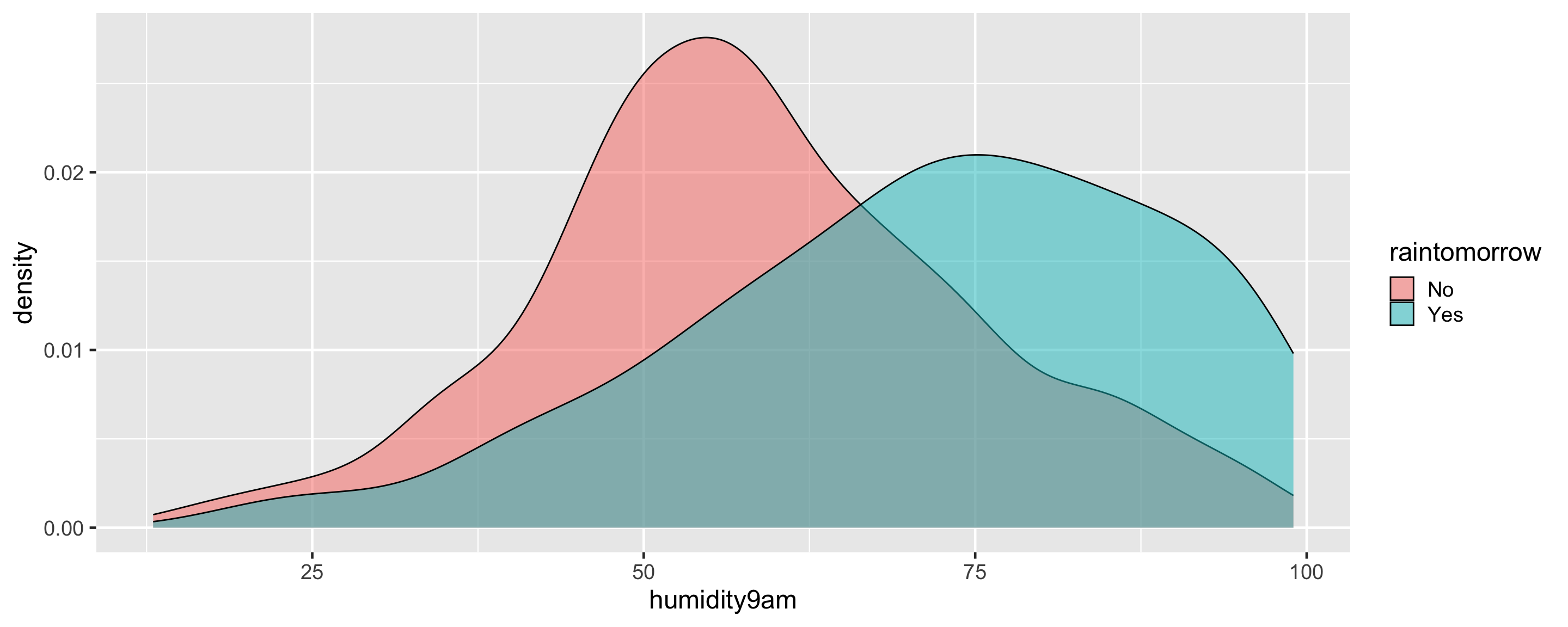
Odds and Probability
\[\text{odds} = \frac{\pi}{1-\pi}\]
if prob of rain = \(\frac{2}{3}\) then \(\text{odds of rain } = \frac{2/3}{1-2/3} = 2\)
if prob of rain = \(\frac{1}{3}\) then \(\text{odds of rain } = \frac{1/3}{1-1/3} = \frac{1}{2}\)
if prob of rain = \(\frac{1}{2}\) then \(\text{odds of rain } = \frac{1/2}{1-1/2} = 1\)
Logistic regression model
likelihood: \(Y_i | \pi_i \sim \text{Bern}(\pi_i)\)
\(E(Y_i|\pi_i) = \pi_i\)
link function: \(g(\pi_i) = \beta_0 + \beta_1 X_{i1}\)
logit link function: \(Y_i|\beta_0,\beta_1 \stackrel{ind}{\sim} \text{Bern}(\pi_i) \;\; \text{ with } \;\; \log\left(\frac{\pi_i}{1 - \pi_i}\right) = \beta_0 + \beta_1 X_{i1}\)
\[\frac{\pi_i}{1-\pi_i} = e^{\beta_0 + \beta_1 X_{i1}} \;\;\;\; \text{ and } \;\;\;\; \pi_i = \frac{e^{\beta_0 + \beta_1 X_{i1}}}{1 + e^{\beta_0 + \beta_1 X_{i1}}}\]
\[\log(\text{odds}) = \log\left(\frac{\pi}{1-\pi}\right) = \beta_0 + \beta_1 X_1 + \cdots + \beta_p X_p \; . \]
When \((X_1,X_2,\ldots,X_p)\) are all 0, \(\beta_0\) is the typical log odds of the event of interest and \(e^{\beta_0}\) is the typical odds.
When controlling for the other predictors \((X_2,\ldots,X_p)\), let \(\text{odds}_x\) represent the typical odds of the event of interest when \(X_1 = x\) and \(\text{odds}_{x+1}\) the typical odds when \(X_1 = x + 1\). Then when \(X_1\) increases by 1, from \(x\) to \(x + 1\), \(\beta_1\) is the typical change in log odds and \(e^{\beta_1}\) is the typical multiplicative change in odds:
\[\beta_1 = \log(\text{odds}_{x+1}) - \log(\text{odds}_x) \;\;\; \text{ and } \;\;\; e^{\beta_1} = \frac{\text{odds}_{x+1}}{\text{odds}_x}\]
# A tibble: 2 × 5
  term        estimate std.error statistic  p.value
  <chr>          <dbl>     <dbl>     <dbl>    <dbl>
1 (Intercept)  -4.57     0.375      -12.2  3.39e-34
2 humidity9am   0.0476   0.00532      8.95 3.55e-19
\[\log\left(\frac{\pi}{1-\pi}\right) = \beta_0 + \beta_1 X_1\] . . .
\[\pi = \frac{e^{\beta_0 + \beta_1 X_1}}{1 + e^{\beta_0 + \beta_1 X_1}}\]
Prediction and Classification
weather %>%
  mutate(log_odds = -4.57 + 0.0476 * humidity9am) %>%
  mutate(prob = log_odds/(1+log_odds)) %>%
  select(-humidity3pm)
# A tibble: 1,000 × 6
day_of_year raintomorrow humidity9am raintoday log_odds prob
<dbl> <dbl> <int> <fct> <dbl> <dbl>
1 45 0 55 No -1.95 2.05
2 11 0 43 No -2.52 1.66
3 261 1 62 No -1.62 2.62
4 347 0 53 No -2.05 1.95
5 357 0 65 No -1.48 3.10
6 254 0 84 Yes -0.572 -1.33
7 364 0 48 No -2.29 1.78
8 293 0 51 No -2.14 1.88
9 304 1 47 Yes -2.33 1.75
10 231 1 90 Yes -0.286 -0.401
# ℹ 990 more rowsPrediction and Classification
weather %>%
  mutate(log_odds = -4.57 + (0.0476 * humidity9am)) %>%
  mutate(prob = exp(log_odds)/(1+exp(log_odds))) %>%
  select(-humidity3pm)
# A tibble: 1,000 × 6
day_of_year raintomorrow humidity9am raintoday log_odds prob
<dbl> <dbl> <int> <fct> <dbl> <dbl>
1 45 0 55 No -1.95 0.124
2 11 0 43 No -2.52 0.0742
3 261 1 62 No -1.62 0.165
4 347 0 53 No -2.05 0.114
5 357 0 65 No -1.48 0.186
6 254 0 84 Yes -0.572 0.361
7 364 0 48 No -2.29 0.0924
8 293 0 51 No -2.14 0.105
9 304 1 47 Yes -2.33 0.0884
10 231 1 90 Yes -0.286 0.429
# ℹ 990 more rowsPrediction and Classification
If we have values for \(\pi\) then we can use these values to predict \(\hat Y\). For instance if \(\pi\) is 0.128 then Y would be randomly sampled from \(\text{Bern}(0.128)\).
set.seed(20641)
weather <- weather %>%
  mutate(log_odds = -4.57 + 0.0476 * humidity9am) %>%
  mutate(prob = exp(log_odds)/(1+exp(log_odds))) %>%
  select(-humidity3pm) %>%
  mutate(y_hat = rbinom(1000, size = 1, prob = prob))

weather
# A tibble: 1,000 × 7
day_of_year raintomorrow humidity9am raintoday log_odds prob y_hat
<dbl> <dbl> <int> <fct> <dbl> <dbl> <int>
1 45 0 55 No -1.95 0.124 0
2 11 0 43 No -2.52 0.0742 0
3 261 1 62 No -1.62 0.165 0
4 347 0 53 No -2.05 0.114 0
5 357 0 65 No -1.48 0.186 0
6 254 0 84 Yes -0.572 0.361 0
7 364 0 48 No -2.29 0.0924 0
8 293 0 51 No -2.14 0.105 1
9 304 1 47 Yes -2.33 0.0884 0
10 231 1 90 Yes -0.286 0.429 1
# ℹ 990 more rowsSensitivity, specificity, and overall accuracy
A confusion matrix summarizes the results of these classifications relative to the actual observations where \(a + b + c + d = n\):
| \(\hat{Y} = 0\) | \(\hat{Y} = 1\) | |
|---|---|---|
| \(Y = 0\) | \(a\) | \(b\) |
| \(Y = 1\) | \(c\) | \(d\) |
\[\text{overall accuracy} = \frac{a + d}{a + b + c + d}\]
\[\text{sensitivity} = \frac{d}{c + d} \;\;\;\; \text{ and } \;\;\;\; \text{specificity} = \frac{a}{a + b}\]
![]()